Categories
Books Coding R

The Monty Hall Problem

I just finished the book “The Monty Hall Problem” by Jason Rosenhouse, which is an exploration of one of the most counter intuitive puzzles in probability. The entire book is devoted to the basic form of the problem and a number of variations, of increasing complexity.

The basic outline of the problem is as follows. You are on a game show and are presented with three closed doors. Behind one of the doors is a prize (say a car) and behind the other two doors is nothing. You are asked to select a door. Once you have picked one of the three doors, the game show host (Monty) opens one of the other doors to reveal that it is empty. Your choice is then to either stick with the door you have initially selected or to change your selection to the other unopened door.

So for example, say you select door 1 below and Monty opens door 2. He then offers you the choice to switch to door 3 or stay with your original selection door 1. You have a choice of two unopened doors. Does it make any difference if you switch or stay?

Most people, myself included, will intuitively say no – there are two doors, and the prize has an equal probability of being behind either of the two remaining doors, so the probability is $\frac{1}{2}$ – switching or sticking makes no difference to the odds of winning the prize. However, this is not the case. Switching to the remaining unopened door will result in a win with a probability of $\frac{2}{3}$. This is a very surprising result and in order to understand why we need to look at the mechanics of the game.

We can prove this very quickly using a simulated approach. If we define the rules of the game as follows:

  • The prize can be behind any door with equal initial probability;
  • Monty will never open the door containing the prize;
  • When Monty has a choice of 2 (empty) doors to open, he will randomly choose between them.

Here is a simple R function that we can use to execute a single run of the game. It simulates the simple game given the rules above, and returns a string describing the winning strategy for that game. For example it will return “Stick” if the winning strategy for that game is to stay with the door you initially selected.

classic_monty <- function() {
  # Assign the prize
  prize <- sample(1:3,1)
  # Pick a door
  choice <- sample(1:3,1)
  # Monty picks a door
  monty <- sample(c(1:3)[-c(choice,prize)], 1)
  return(ifelse(prize!=choice, "Switch", "Stick"))
}

We can run the game a few times and see the result:

> classic_monty()
[1] "Switch"
> classic_monty()
[1] "Stick"
> classic_monty()
[1] "Switch"

To see the asymptotic win probability of switch or stick, we can replicate the experiment a number of times and record the outcome:

n <- 2^(1:16)
runs <- data.frame(n=numeric(), switch=numeric())
for (trials in n) {
  run <- table(replicate(trials, classic_monty()))
  runs <- runs %>%  add_row(n=trials, switch=(sum(run["Switch"]))/trials)
}
# Handle zero-occurrence trials
runs[is.na(runs)]<-0

If we run this, then we can examine the win probability using the switch strategy as we increase the number of trials:

> runs
       n    switch
1      2 0.0000000
2      4 0.2500000
3      8 0.6250000
4     16 0.5000000
5     32 0.5937500
6     64 0.7031250
7    128 0.6640625
8    256 0.6835938
9    512 0.6484375
10  1024 0.6640625
11  2048 0.6748047
12  4096 0.6645508
13  8192 0.6702881
14 16384 0.6721191
15 32768 0.6636963
16 65536 0.6641541

There is a clear convergence to a $\frac{2}{3}$ win probability using the switch strategy. This is something I had to simulate to initially accept, as my intuitive expectation was a win probability of $\frac{1}{2}$.

In order to understand the mechanics behind this result a little more, we can generate the full space of possible outcomes $ \left( C, M, P\right) $for each trial, where $C$ is the door we choose, $M$ is the door Monty opens, and $P$ is the door that hides the prize. For example the tuple $\left( 1, 2, 3\right)$ would be the scenario where we pick door 1, Monty reveals door 2, and the prize sits behind door 3.

The code to generate the sample space is below:

# Generate sample space of tuples for Monty-Hall 
space <- data.frame(choice=numeric(), monty=numeric(), prize=numeric())

i <- 1
for (prize in 1:3) {
 for (choice in 1:3) {
    for (monty in c(1:3)[-c(prize,choice)]) {
      space <- space %>%  add_row(choice=choice,monty=monty,prize=prize)
    }
  }
}

space <- space %>% arrange(choice)

Which will generate a table as follows:

> head(space)
  choice monty prize
1      1     2     1
2      1     3     1
3      1     3     2
4      1     2     3
5      2     3     1
6      2     1     2

Let’s look at a sample play. Say we choose door 1. The sample space for possible plays where we choose door 1 is:

1      1     2     1
2      1     3     1
3      1     3     2
4      1     2     3

So if we stick with door 1 it looks like we have 2 outcomes out of 4, or a 50% chance of winning. However this is not the case, as the first two rows in the sample space above must have the same probability as each of the last two rows – door 1 has a fixed probability of $\frac{1}{3}$ of hiding the prize and that cannot change. So the first two outcomes above have a combined probability of $\frac{1}{3}$, which means that the win probability when switching is $\frac{2}{3}$.

Once we see the sample space enumerated like this, the reason for the switch probability seems obvious – due to the rules of the game outlined above, we have constrained the sample space. If the host follows the rules above and randomly chooses between two unopened doors when we have selected the door with the prize, but in all other cases will only open the door that is empty, we can see that the choice of door opened by Monty contains information – which is why his choice of door is important.

The Bayesian Approach

As an aside, the book contains a short conditional probability-based approach to the simple scenario above that I think is worth showing. If $C_n$ denotes that the prize is behind door $n$ and $M_m$ denotes that Monty opens door $m$, then assuming we choose door 1 as above and Monty then opens door 2 – we can ask the question what is the probability now that the prize is behind door 3 – i.e. $P(C_3|M_2)$?

This is $P(C_3|M_2) = \frac{P(M_2|C_3)P(C_3)}{P(M_2)}$

$=\frac{P(M_2|C_3)P(C_3)}{P(M_2|C_1)P(C_1)+P(M_2|C_2)P(C_2)+P(M_2|C_3)P(C_3)}$

We can infer that if any door is initially likely to contain the prize, then

$P(C_1)=P(C_2)=P(C_3)=\frac{1}{3}$

And as Monty will not open the door hiding the prize $P(M_2|C_2)=0$, and will be forced to open the only remaining door if we have chosen door 1 and the prize is behind door 3, then $P(M_2|C_3)=1$

This then simplifies to

$P(C_3|M_2) = \frac{1}{P(M_2|C_1)+1}$

We can figure out $P(M_2|C_1)$ using the simple rules of the game – if we have selected door 1 and the prize is behind door 1, Monty must choose randomly between the other two doors. So $P(M_2|C_1)=P(M_3|C_1)=\frac{1}{2}$.

Thus

$P(C_3|M_2) = \frac{2}{3}$

Another nice approach. This is a nice problem to illustrate just how deceptive simple probability puzzles can be!

Categories
Coding R

The Mandelbrot Set

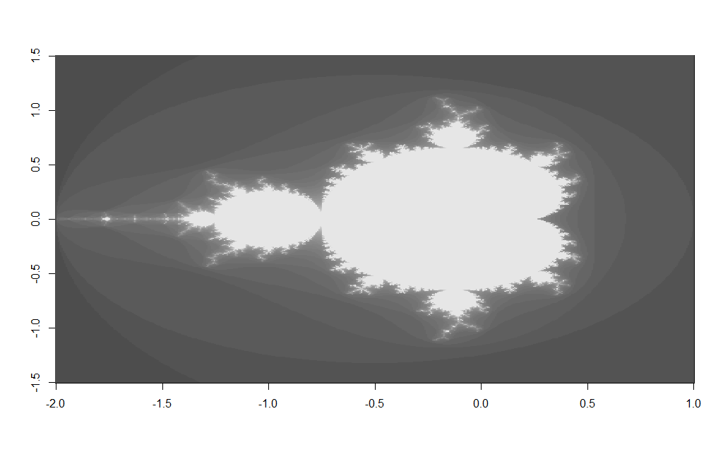
The Mandelbrot Set is possibly one of the most visually appealing mathematical visualizations. The set is defined as the set of complex numbers $c$ for which the function $f_c(z) = z^2 + c$ remains bounded when iterated – i.e. the sequence $f_c(z), f_c(f_c(z)),f_c(f_c(f_c(…)))$ remains bounded below some fixed absolute threshold.

The basic method to generate a simple Mandelbrot set is fairly simple:

  • Choose the values of $c$ to put in the iteration $z\rightarrow z^2+c$;
  • Iteratively apply the mapping for each value of $c$ and test if the updated value is now $\geq \epsilon$ where $\epsilon$ is some fixed absolute threshold;
  • Update our output grid to reflect the intensity at point $c$ – this can be a simple 1/0 to indicate that the iteration has become unbounded (or ‘escaped’) or it can be a value reflecting how many iterations it took before the value was determined to escape (or not)

R has a ‘native’ representation for complex numbers but for this example we will just use a 2-element vector as a complex number representation, each element being the real and imaginary components respectively.

The iterative step at each point to update the current value of $z \rightarrow z^2+c$ is computed as follows – if $z$ is assumed to be a complex number of the form $x+yi$:

$$(x+yi)(x+yi) = x^2-y^2+2xyi$$

So $Re(z)\rightarrow x^2-y^2+Re(c) $ and $Im(z) \rightarrow 2xy+Im(c)$

Here is some simple R code to illustrate:

# Subset of x-y plane
x <- c(-2,1)
y <- c(-1.5, 1.5)

# Number of points in each dimension
nx <- 500
ny <- 500

xgrid <- seq(x[1],x[2], length.out = nx)
ygrid <- seq(y[1],y[2], length.out = ny)


mand <- function(xgrid,ygrid,frac) {
  i <- j <- it <- 1
  z <- c <- zprev <- c(0,0)
  TOL <- 4  # Escape value
  N <- 50   # Number of iterations to test for escape
  # The output fractal trace
  frac <- matrix(nrow=nx, ncol=ny, byrow=TRUE)
  
  for (i in seq_along(xgrid)) {
    for (j in seq_along(ygrid)) {
      c <- c(xgrid[i],ygrid[j])  
      z <- c(0,0)
      
      for (k in 1:N) {
        it <- k
        zprev <- z
        # If zprev is a complex number x + yi
        # Then we update z as follows:
        # Re(z) <- (x^2-y^2) + Re(c)
        z[1] <- zprev[1]*zprev[1]-zprev[2]*zprev[2]+c[1]
        # Im(z) <- 2*z*y + Im(c)
        z[2] <- 2*zprev[1]*zprev[2]+c[2]            
        if ((z[1]*z[1] + z[2]*z[2])>TOL) { break }
      }
      frac[i,j] <- it
    }
  }
  
  return(list(x=xgrid,y=ygrid,z=frac))
}

To call the function and plot the output:

m <- mand(xgrid,ygrid,frac)
image(m, col=gray.colors(50)) 

Which should produce an image like the following:

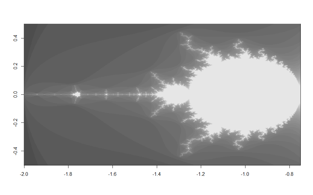
Changing the $x$ and $y$ grid coordinates enables you too zoom in to various areas on the fractal e.g. changing the x/y grid to:

x <- c(-2,-0.75)
y <- c(-0.5, 0.5)

Results in the image below

The main drawback of iterative plain R code like this is that it is slow – however this could be speeded up using a native interface e.g. Rcpp and computing the iterative process in C/C++ code, where some of the copying overhead may be avoided.

Categories
Coding Finance R Statistics

Fooled By Randomness

I recently read the great book Fooled By Randomness by Nicholas Nassim Taleb. There is a nice illustrative example in there on the scaling property of distributions across different time scales. The example is formulated as the hypothetical example of a dentist who has set up a home trading environment and started to invest in some assets (say stocks). The dentist has access to real-time market data and thus can check in on their current investment portfolio valuation at any point in time.

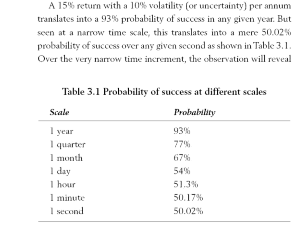
The investment portfolio has an expected annual return of 15% and volatility of 15%. The assertion in the book is that the more frequently the dentist appears to check the performance of the portfolio, the worse it will seem to perform(see the table below). The question is why, as at first glance it appears counter-intuitive.

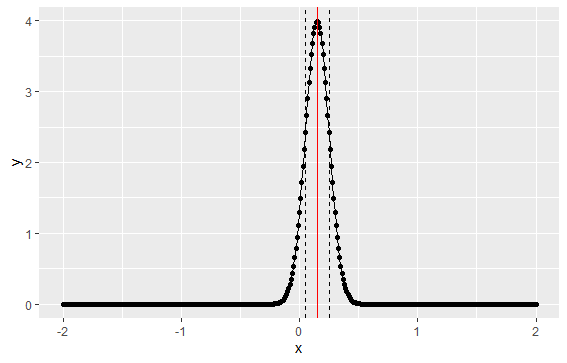
The answer is as follows – if we assume a normal distribution for the portfolio returns, the parameters above define a distribution with a mean of 15% and a standard deviation of 10%, .i.e. $\mathcal{N}(0.15, 0.10)$

We can represent this in R as follows:

mu <- .15
sigma <- .1
x <- seq(-2,2,.01)
y <- dnorm(x,mean = mu, sd = sigma)
qplot(x,y) + geom_line() + geom_vline(aes(xintercept=mu),color='red') + geom_vline(aes(xintercept=c(mu-sigma,mu+sigma)),linetype=2)

The graph shows the implied distribution plus the mean (red line) and standard deviation (dashed lines)

Under this implied distribution, 2 standard deviations (or 95%) results in a return spanning -5% to +35%:

mu + 2*sigma
[1] 0.35
mu - 2 *sigma
[1] -0.05

Looking again at the table from the book above – if we calculate success as a return > 0, then we can calculate the probability of success for the distribution above. We can calculate this using the the normal cumulative distribution – which is basically the the sum of the area under the normal curve above – and find out what this value is for 0.

In R, pnorm() gives us the area under the curve. Actually it gives us $P(X<=0)$ so in order to calculate success $(P(X>0))$ we need to calculate the inverse probability:

1-pnorm(0,mean = mu, sd=sigma)
[1] 0.9331928

So the probability of success over one year is 93%, which matches the table above.

Now what happens if the dentist checks their portfolio more frequently – i.e. what does the return look like over 1 quarter as opposed to 1 year? In order to calculate this, we need to adjust the parameters to scale it to a quarterly distribution. So $\mu_Q = \frac{\mu_A}{4}$ and $\sigma_Q = \frac{\sigma_A}{\sqrt{4}}$, i.e. the mean will be divided by 4 to convert to quarters, and the standard deviation will be divided by the square root of 4, as volatility scales with the square root of time.

1-pnorm(0,mean = mu/4, sd=sigma/sqrt(4))
[1] 0.7733726

So we can see that moving from an annual to a quarterly distribution has lowered the probability of success from 93% to 77%

Similarly if we now move from quarterly to monthly, the distribution will be a $ \mathcal{N}{\frac{\mu_A}{12}, \frac{\sigma_A}{\sqrt{12}}}$ distribution:

1-pnorm(0,mu/12, sigma/sqrt(12))
[1] 0.6674972

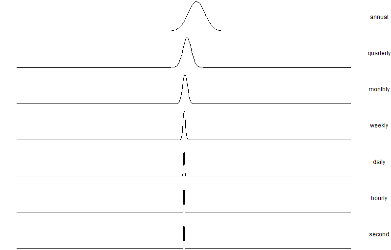
Which is roughly 67%. Further, we can tabulate the various scaling factors all the way from 1 (annual) to 31536000 (1-second horizon) and calculate the probability of success for each time horizon. We can see the success probability diminish from 93% down to 50% at a one-second resolution.

factors <- c(1,4,12,52,365,8760,31536000)
sapply(factors, function(x) success(mu, sigma, x))
[1] 0.9331928 0.7733726 0.6674972 0.5823904 0.5312902 0.5063934 0.5001066

To make it clearer we can calculate the density of each distribution and plot it:

mu <- 0.15
sigma <- 0.1
x <- seq(-2,2,.01)
factors <- c(1,4,12,52,365,8760,31536000)
names <- c('x','annual','quarterly','monthly','weekly','daily','hourly','second')

# Calculate the density for the distribution at each timescale 
tab <- data.frame(x=x)
for (f in seq_along(factors)) {
  tab <- cbind(tab, dnorm(x, mu/factors[f], sd=sigma/sqrt(factors[f])))
}

# Plot each density in a separate panel
colnames(tab) <- names
ggplot(melt(tab,id.vars = 'x'), aes(x=x)) + geom_line(aes(y=value)) + facet_grid(variable~.,scales = 'free') + xlab('') + ylab('') + theme_void() + theme(strip.text.y = element_text(angle = 0))