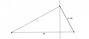
Here’s a simple and intuitive way of looking at the geometry of a least squares regression:
Take the bottom left point in the triangle below as the origin O. For the linear model:
$$ Y=X\beta + \epsilon $$
Both $Y$ and \(X\beta\) are vectors, and the residual vector \(\epsilon\) is the difference. The standard least squares error technique uses \(\epsilon^2\) or \((Y-X\beta)^T(Y-X\beta)\) as the error measure to be minimised, and this leads to the calculation of the \(\beta\) coefficient vector.

Geometrically, the beta coefficients calculated by the least squares regression minimise the squared length of the error vector. This turns out to be the projection of \(Y\) on to \(X\beta\) – i.e. the perpendicular vector that turns (O, \(Y\), \(X\beta\)) into a right-angled triangle.
The projection of \(Y\) onto \(X\beta\) is done using the projection matrix P, which is defined as
\[ P = X\left(X^{T}X\right)^{-1}X^{T} \]
So \( X\beta = \hat{Y} = PY \).
Using the Pythagorean theorem:
\( Y^TY = \hat{Y}^T\hat{Y} + (Y-X\beta)^T(Y-X\beta) \)
In other words, the total sum of squares = sum of squares due to regression + residual sum of squares. This is a fundamental part of analysis of variance techniques.