Random number generation is a core topic in numerical computer science. There are many efficient
algorithms for generating random (strictly speaking, pseudo-random) variates
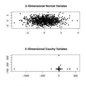
from different probability distributions. The figure below shows a
sampling of 1000 two-dimensional random variates from the standard Gaussian and
Cauchy distributions, respectively. The size of the extreme deviations of the
Cauchy distribution is apparent from the graph.
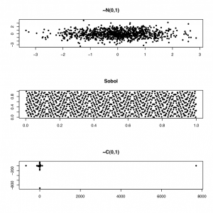
However, sometimes we need to produce numbers that are more evenly distributed (quasi-random numbers). For example, in a Monte Carlo integration exercise, we can get faster convergence with a lower error bound using so-called low-discrepancy random sequences, using the GSL library. In the figure below, we show two-dimensional normal and Sobol (a low-discrepancy generator) variates.

To generate the graph below, I used the GSL library for R, as shown below:
[source lang=”R”]
library(gsl)
q <- qrng_alloc(type="sobol", 2)
rs <- qrng_get(q,1000)
par(mfrow=c(3,1))
plot(rnorm(1000), rnorm(1000), pch=20, main="~N(0,1)",
ylab="", xlab="")
plot(rs, pch=20, main="Sobol",
ylab="", xlab="")
plot(rcauchy(1000), rcauchy(1000),pch=20,
main="~C(0,1)", ylab="",xlab="")
[/source]
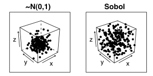
The property of low-discrepancy generators is even more apparent if we view the random variates in a higher dimension, for example the figure below shows the variates as a 3-dimensional cube. Note how the clustering around the centre of the cube is much more pronounced for the Gaussian cube.

To plot the figure above, I used the GSL and Lattice libraries:
[source lang=”R”]
library(gsl)
library(lattice)
q <- qrng_alloc(type="sobol", 3)
npoints <- 200
rs <- qrng_get(q,npoints)
ltheme <- canonical.theme(color = FALSE)
ltheme$strip.background$col <- "transparent"
lattice.options(default.theme = ltheme)
trellis.par.set(layout.heights =
list(top.padding = -20,
main.key.padding = 1,
key.axis.padding = 0,
axis.xlab.padding = 0,
xlab.key.padding = 0,
key.sub.padding = 0,
bottom.padding = -20))
# Plot the normal variates in a 3-dim cube
p1 <- cloud(rnorm(npoints) ~ rnorm(npoints) + rnorm(npoints), xlab="x", ylab="y",
zlab="z", pch=20, main="~N(0,1)")
p2 <- cloud(rs[,1] ~ rs[,2] + rs[,3], xlab="x", ylab="y",
zlab="z", pch=20, main="Sobol")
print(p1, split=c(1,1,2,1), more=TRUE)
print(p2, split=c(2,1,2,1))
[/source]
