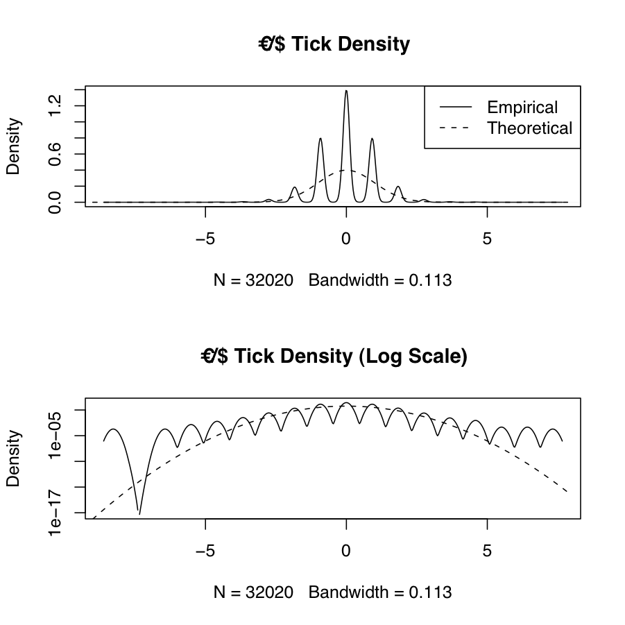
Density Estimation of High-Frequency Financial Data

Frequently we will want to estimate the empirical probability density function of real-world data and compare it to the theoretical density from one or more probability distributions. The following example shows the empirical and theoretical normal density for EUR/USD high-frequency tick data $X$ (which has been transformed using log-returns and normalized via $\frac{X_{i} - μ_{X}}{σ_{X}}$ ). The theoretical normal density is plotted over the range $(⌊ \min (X) ⌋, ⌈ \max (X) ⌉)$ . The results are in the figure below. The discontinuities and asymmetry of the discrete tick data, as well as the sharp kurtosis and heavy tails (a corresponding interval of $\approx [- 8, + 7]$ standard deviations away from the mean) are apparent from the plot.

tick density — Empirical and Theoretical Tick Density

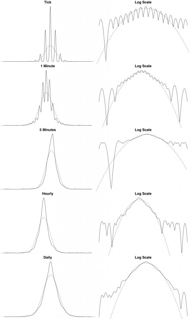
We also show the theoretical and empirical density for the EUR/USD exchange rate log returns over different timescales. We can see from these plots that the distribution of the log returns seems to be asymptotically converging to normality. This is a typical empirical property of financial data.

density_scaled — Density Estimate Across Varying Timescales

The following R source generates empirical and theoretical density plots across different timescales. The data is loaded from files that are sampled at different intervals. I cant supply the data unfortunately, but you should get the idea.

[source lang=”R”]
# Function that reads Reuters CSV tick data and converts Reuters dates
# Assumes format is Date,Tick
readRTD <- function(filename) {
tickData <- read.csv(file=filename, header=TRUE, col.names=c("Date","Tick"))
tickData $D a t e < - a s . P O S I X c t (s t r p t i m e (t i c k D a t a$ Date, format="%d/%m/%Y %H:%M:%S"))
tickData
}

# Boilerplate function for Reuters FX tick data transformation and density plot
plot.reutersFXDensity <- function() {
filenames <- c("data/eur_usd_tick_26_10_2007.csv",
"data/eur_usd_1min_26_10_2007.csv",
"data/eur_usd_5min_26_10_2007.csv",
"data/eur_usd_hourly_26_10_2007.csv",
"data/eur_usd_daily_26_10_2007.csv")
labels <- c("Tick", "1 Minute", "5 Minutes", "Hourly", "Daily")

par(mfrow=c(length(filenames), 2),mar=c(0,0,2,0), cex.main=2)
tickData <- c()
i <- 1
for (filename in filenames) {
tickData[[i]] <- readRTD(filename)
# Transform: ` $Y = \nabla \log (X_{i})$ `
logtick <- diff(log(tickData[[i]] $You can't use 'macro parameter character #' in math mode$ \frac{(Y-\mu_Y)}{\sigma_Y} $You can't use 'macro parameter character #' in math mode$ \left[\lfloor\mathrm{min}(Y)\rfloor,\lceil\mathrm{max}(Y)\rceil\right]$`
x <- seq(floor(min(logtick)), ceiling(max(logtick)), .01)
plot(density(logtick), xlab="", ylab="", axes=FALSE, main=labels[i])
lines(x,dnorm(x), lty=2)
#legend("topleft", legend=c("Empirical","Theoretical"), lty=c(1,2))
plot(density(logtick), log="y", xlab="", ylab="", axes=FALSE, main="Log Scale")
lines(x,dnorm(x), lty=2)
i <- i + 1
}
par(op)
}
[/source]