Introduction
In economics, the Gini Coefficient (http://www.statistics.gov.uk/about/methodology_by_theme/gini/default.asp) is a standard quantitative measure of the relative inequality in the distribution of wealth. The name “Gini Coefficient” is a moniker for a large family of variations on the basic inequality measure, but the standard interpretation is that of the ratio of the area under the Lorenz curve (a function of the cumulative distribution) to that of the line of perfect equality. The coefficient is normalized such that it lies between 0 and 1, where 0 represents perfect equality (for example, everyone has the same amount of wealth), and 1 represents perfect inequality (one person holds all of the wealth). For instance, say we have a theoretical population where everyone has the same income, say $100. If we are using R, we can calculate the Gini coefficient (using the ineq library):
>library(ineq)

> x < - rep(100,10)
> x

 [1] 100 100 100 100 100 100 100 100 100 100

> round(Gini(x))

[1] 0

> plot(Lc(x))

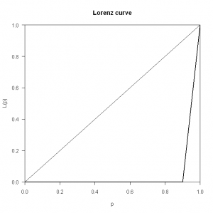
Now if we create a theoretical income distribution where one member (or class) earns $100 and everybody else earns nothing, we have perfect inequality:
> x < - c(100,rep(0,9)) > x
[1] 100 0 0 0 0 0 0 0 0 0
> round(Gini(x))
[1] 1
> plot(Lc(x))

But what has this got to do with software?
At the User! 2008 conference in Germany this year, John Fox gave a superb talk on the social construction of the R project. The talk was very interesting for a number of reasons, but mainly because he looked at the project’s evolution not from the standard technical viewpoint that we tend to unconsciously fall into, but rather from the viewpoint of that of a qualitative social scientist. The result was a fascinating exposition of the social dynamics behind an extremely popular and large open source project (The slides for John’s talk are available online from the conference site here).
One surprising fact that John revealed in his presentation was the relative dependence of the R project (which has a core team of around 20 members) on a single individual committer. To quantify this, John calculated the Gini coefficient for the R project, where the inequality metric was based on the number of commits per core team member (extracted from the R svn logs). The results were surprising – a Gini coefficient of over 0.8, which signifies a large degree of inequality in the number of commits per member. This may signify a large dependence on a single member of the project team, a situation referred to in management-speak as “key man risk”.
We can reproduce this analysis using R and a copy of the R svn commit logs (found here). In order to turn the output of svn log into something we can work with, we need to massage the data slightly. I just did this in Vim, using the two commands:
%v/^r\d\+\s\+|/d
To remove all lines that we are not interested in, followed by
%s/^r\(\d\+\)\s\+|\s\+\(\w\+\)\s\+|\s\+\(\d\+-\d\+-\d\+ \d\+:\d\+:\d\+\) .*/\1,\2,\3/
to turn the log output into a comma-delimited triplet of revision number, author, and date. To load it into R, I used read.table():
R_svn < - read.table("/tmp/R_svnlog_2008.dat", col.names=c("rev","author","date"),sep=",")
As R will turn repeated string data (such as the committer name) into a factor, it is trivial to extract the data we need to calculate the Gini coefficient using a contingency table:
> round(Gini(table(R_svn$author)), 2)

[1] 0.81
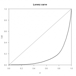
And then plot the Lorenz curve:

As you can see, the curve is skewed towards large inequality. The (possibly) worrying aspect of this metric is that it is increasing over time (as illustrated in John Fox’s presentation), signifying that dependence on a single team member is growing.
What’s The Problem With This Metric?
So is this actually meaningful – i.e. is there anything to be concerned about in this measure? Well, for starters, there are a few obvious drawbacks with this metric. One primary flaw is that the number of commits per developer is a weak measure if we take it to signify total contribution towards a project. Some developers prefer to commit smaller changes more often, whilst others prefer to commit larger, more complete changes less frequently. The number of commits is also completely independent from the quality of those commits. Another crucial factor is that committing code is just one part of the work that goes into a successful open source project. Other tasks include, but are not limited to: website maintenance, release management, mailing list participation and support, and general advocacy and awareness tasks. A blunt metric such as number of commits per developer will not take any of these into account.
Improving The Metric
Due to the nature of software development, no single quantitative measure will be able to accurately describe a complete measure of contribution. However, if we were to try and improve on the basic commit metric, we could conceivably propose something like the following:
\[C = \beta_1 \lambda(N_C) + \beta_2 \lambda(N_L) + \beta_3 \lambda(N_I) + \beta_4 \lambda(N_M)\]
Where the <\(\beta\) components are just weights applied to each factor, and the factors are:
- \(N_C\): Number of commits;
- \(N_L\): Number of source lines changed;
- \(N_I\): Number of issues or bugs closed/resolved/participated in;
- \(N_M\): Number of messages posted to e.g. a user mailing list
The \[\lambda\] function is just an exponential decay factor, to compensate for the survivor bias inherent in such statistics. Most of these numbers are reasonably easily obtainable for open source projects. Such a metric would probably be more informative than the simple “commits per developer” model, in that it would provide a slightly more balanced notion of “contribution”.
Some Other Examples
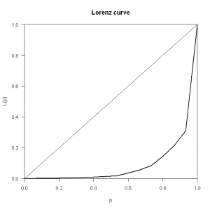
Just out of curiosity, I decided to calculate the coefficient for some other large software projects, including Apache httpd and Parrot (Perl 6). The results for Parrot are shown below:
> round(Gini(table(parrot_svn$author)),2)

[1] 0.74

Parrot exhibits a few of the features that seem to be common to many open source projects: the commit distribution is mainly peaked at the low end, with a smaller set of peaks at the high end, signifying that most project members make a relatively small number of commits, but an individual or small core group of individuals make a much larger set of commits. This makes perfect sense: project founders, so-called “benevolent dictators”, developers in the employ of companies who contribute to open source projects, or simply developers with more time and energy on their hands will contribute the lion’s share of the project effort. In a commercial enterprise, this may be more of a concern (due to the time and cost implications of sudden replacement) than in open source projects, where by definition, the openess of the codebase and contribution process offers a buffer against adverse consequences of key man risk.